AfD 2017 election results, incidence rates, and vaccinations
By Manuel Rademaker in Data Science Covid 19 SARS-COV2 2017 Election R Maps Interactivity
August 31, 2021
Recently, I stumbled across this graphic from great KATAPULT magazin:
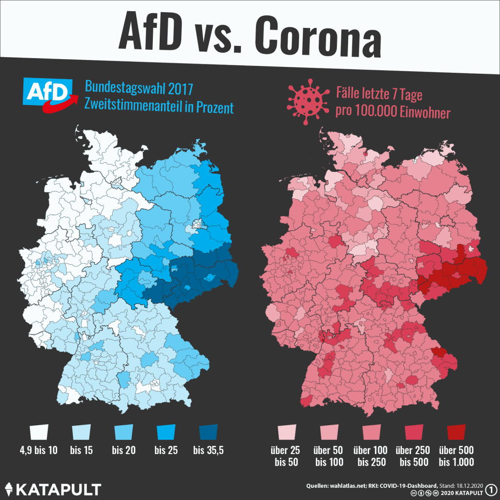
The left map shows the final 2017 parliamentary election (second vote) results (Zweitstimmenergebnis Bundestagswahl 2017) by election region (Wahlkreis) for the German party “Alternative für Deutschland” (AfD). On the right, the 7-day COVID-19 incidence per 100,000 people is shown by administrative region (Landkreis) as of 18.12.2020. Note that Wahlkreise and Landkreise are generally similar but do differ on many occasions.
What the graphic suggests is a correlation (visually quite a pronounced one!) between the 2017 election results and the 7-day incidence: the more people voted for the AfD in 2017, the higher the incidence. I found this visualization pretty telling, although, to be fair, I suspect the date (18.12.2020) was most likely chosen such that the correlation is most striking and, as usual, causation cannot be inferred from correlation without context. Of course, the authors of the visualization know about the difference between correlation and causation. They write on their website:
“Ob der Zusammenhang kausal ist, also ein Ursache-Wirkungs-Zusammenhang besteht, ist unklar” (“Whether the relationship is causal, i.e. there is a cause-effect relationship, is unclear”).
No matter the question of correlation vs. causation or the political implications a truly causal relationship would have, I took this graphic as an opportunity to learn more about COVID-19 data and to keep practicing my data analysis skills general. Most notably, I am interested in:
- the relationship between election results and commonly used SARS-COV-2/COVID-19 indicators such as the 7-day incidence or the vaccination rate. I’m particularly interested to see if there is a similar relationship between election results (for the AfD or other parties) and vaccination rates by Landkreis or if there is a similar relationship between incidence and election results for other parties as well.
- data processing in general: in particular making maps in R, pulling data from different sources, cleaning, merging and everything else needed to create meaningful visualizations – quite in the spirit of my TidyTuesday Series.
Setup
To follow along, download the file xxx containing the R script. Make sure you have the following packages installed and load them.
require(tidyverse)  # tidyverse packages
require(scales)     # formating numbers
require(sf)         # working with shape files
require(readr)      # fast reading of csv files
require(gt)         # create nice-looking tables
require(patchwork)  # combine plots
require(glue)       # Glue strings to data in R
require(ggiraph)    # Create interactive graphs
require(zoo)        # to compute the rolling 7-day sum
require(xts)        # for working with time series
require(dygraphs)   # interactive time series
A note for those wondering
I know about the
COVDID-19 Data Hub
which contains a ton of COVID-19 related info across countries and administrative areas.
Moreover, there are numerous projects that provide COVID-19 related data or APIs
to that data in a clean, curated way (e.g.,
here
and
here).
The reason I do not use any of those sources is twofold. First, I consider writing
this blog post more as an exercise. Taking a curated data
set would be like taking a shortcut when you are going for a hike – it simply
misses the point. Second, the R package COVID19 – an interface to the COVID-19 Data Hub –
does not provide vaccination data on the Landkreis level, so I decided to use the raw RKI data. While the package does provide infection
data, it does not contain the AGS (“Amtlicher Gemeindeschlüssel”). The AGS is essentially a
unique Id for each Landkreis and kreisfreie Stadt that is used by all official/administrative data
providers. Since I need to match different data sets by Landkreis later, its nice
to have an Id since matching by Id is a lot – backed by (bad) experiences – less error-prone
than by name. Moreover, the AGS has the added benefit of a clear
hierarchical structure that allows easy identification of adherence of e.g. a
Landkreis or Gemeinde to other administrative areas such as its corresponding Bundesland.
Hence, I decided I go with the official data.
That being said, still do check out the COVID19 package website as it can be super helpful for other COVID-19/SARS-COV-2 related questions.
Data
Getting the data
I use different data throughout this post. For clarity, I list all data including
their source and a direct link that will automatically start a download in a table here.
If you want to follow along, download the first three datasets/zip-files,
unzip (if necessary) and put the raw data or folders containing the data in the same folder as the
R script and rename (if necessary) the files according to the Name column.
For the RKI data, it is easiest to just provide the data link to read_csv() directly without
downloading the .csv file first (see below).
Note:
- Wahlkreise can change from election to election. The shapefile below is the version relevant for the 2017 election. To get the version relevant for the 2021 election click here.
- The data from RKIs GitHub page is updated on a daily basis. If you want
to reproduce the exact numbers of this post, only use dates smaller than 2021-08-31. - As I mentioned in my note above: learning about data processing is part of the exercise. Hence, I deliberately only use raw data from the original sources.
| File name | Source / Direct link | Description |
|---|---|---|
election_results_2017.csv |
Bundeswahlleiter, Direct-link-to-data | Final results of the 2017 general election by Wahlkreis. |
wahlkreise_shp_2017.zip |
Bundeswahlleiter, Direct-link-to-data | .zip file containing the geometry for all 299 Wahlkreise in different formats. In the following, I only use the shapefile format (.shp). The file needed is called: Geometrie_Wahlkreise_20DBT_VG250_geo.shp. |
vg250_ew_2020.zip |
BfKG, Direct-link-to-data | .zip file containing the geometry of German administrative areas including population from the “Bundesamt für Kartografie und Geodäsie” as of 01.01.2020. Only the geometry of the Kreise and kreisfreie Städte is needed. The relevant file is called: VG250_KRS.shp. |
Aktuell_...-Impfungen.csv |
RKI GitHub, Direct-link-to-data | Absolute number of people vaccinated against COVID-19 by Landkreis, date, age group, and vaccination number (first or second) starting 27.12.2020. |
Aktuell_..._Infektionen.csv |
RKI Github, Direct-link-to-data | Absolute number of infections with the SARS-COV-2 virus by Landkreis, date, age group and other characteristics. |
Reading the data
Once you have downloaded and unzipped the data, run the following to read the data into R. Ignore all the warnings and messages. We will have to do some processing anyway.
# 2017 German parliamentary election results
election_results_2017 <- read_csv2("election_results_2017.csv", skip = 5)
# Shapefile with the geometry of the 299 german Wahlkreise
wahlkreise_shp_2017   <- st_read("wahlkreise_shp_2017/Geometrie_Wahlkreise_20DBT_VG250_geo.shp")
# Shapefile with the geometry (including population) of the 401 Landkreise and kreisfreie Städte
vg250_ew_2020         <- st_read("vg250_ew_2020/vg250-ew_12-31.gk3.shape.ebenen/vg250-ew_ebenen_1231/VG250_KRS.shp")
# Absolute number of people vaccinated by characteristics
vaccinated_raw <- read_csv("https://raw.githubusercontent.com/robert-koch-institut/COVID-19-Impfungen_in_Deutschland/master/Aktuell_Deutschland_Landkreise_COVID-19-Impfungen.csv")
# Absolute number SARS-COV-2 infections by characteristics
infections_raw <- read_csv("https://media.githubusercontent.com/media/robert-koch-institut/SARS-CoV-2_Infektionen_in_Deutschland/master/Aktuell_Deutschland_SarsCov2_Infektionen.csv")
If you prefer the more programmatic approach, you can also skip downloading manually and use R to download, unzip and read the files directly without leaving your R session.
# 2017 german parliamentary election results
election_results_2017_url <- "https://www.bundeswahlleiter.de/dam/jcr/72f186bb-aa56-47d3-b24c-6a46f5de22d0/btw17_kerg.csv"
download.file(election_results_2017_url, destfile = "election_results_2017.csv")
election_results_2017 <- read_csv2("election_results_2017.csv", skip = 5)

# Shapefile with the geometry of the 299 german Wahlkreise
wahl_shp_url <- "https://www.bundeswahlleiter.de/dam/jcr/4238f883-5a9b-4da6-a4d5-ac86f3752b88/btw21_geometrie_wahlkreise_vg250_geo_shp.zip"
download.file(wahl_shp_url, destfile = "wahlkreise_shp_2017.zip")
unzip("wahlkreise_shp_2017.zip", exdir = "wahlkreise_shp_2017")
wahlkreise_shp_2017 <- st_read("wahlkreise_shp_2017/Geometrie_Wahlkreise_20DBT_VG250_geo.shp")
## Reading layer `Geometrie_Wahlkreise_20DBT_VG250_geo' from data source
##   `C:\Users\manue\Dropbox\Desk\R-Projekte\personal-website\content\blog\2021-08-31_election_results_and_covid_data\wahlkreise_shp_2017\Geometrie_Wahlkreise_20DBT_VG250_geo.shp'
##   using driver `ESRI Shapefile'
## Simple feature collection with 299 features and 4 fields
## Geometry type: MULTIPOLYGON
## Dimension:     XY
## Bounding box:  xmin: 5.86625 ymin: 47.27012 xmax: 15.04182 ymax: 55.05838
## Geodetic CRS:  WGS 84
# Shapefile with the geometry (including population) of the 401 Landkreise and kreisfreie Städte
vg250_ew_2020_url <- "https://daten.gdz.bkg.bund.de/produkte/vg/vg250-ew_ebenen_1231/aktuell/vg250-ew_12-31.gk3.shape.ebenen.zip"
download.file(vg250_ew_2020_url, destfile = "vg250_ew_2020.zip")
unzip("vg250_ew_2020.zip", exdir = "vg250_ew_2020")
vg250_ew_2020 <- st_read("vg250_ew_2020/vg250-ew_12-31.gk3.shape.ebenen/vg250-ew_ebenen_1231/VG250_KRS.shp")
## Reading layer `VG250_KRS' from data source
##   `C:\Users\manue\Dropbox\Desk\R-Projekte\personal-website\content\blog\2021-08-31_election_results_and_covid_data\vg250_ew_2020\vg250-ew_12-31.gk3.shape.ebenen\vg250-ew_ebenen_1231\VG250_KRS.shp'
##   using driver `ESRI Shapefile'
## Simple feature collection with 431 features and 28 fields
## Geometry type: MULTIPOLYGON
## Dimension:     XY
## Bounding box:  xmin: 3280359 ymin: 5237511 xmax: 3921536 ymax: 6103443
## Projected CRS: DHDN / 3-degree Gauss-Kruger zone 3
# Absolute number of people vaccinated by characteristics
vaccinated_raw <- read_csv("https://raw.githubusercontent.com/robert-koch-institut/COVID-19-Impfungen_in_Deutschland/master/Aktuell_Deutschland_Landkreise_COVID-19-Impfungen.csv")

# Absolute number SARS-COV-2 infections by characteristics
infections_raw <- read_csv("https://media.githubusercontent.com/media/robert-koch-institut/SARS-CoV-2_Infektionen_in_Deutschland/master/Aktuell_Deutschland_SarsCov2_Infektionen.csv")
Analysis
Election results by Wahlkreis
Lets start by reproducing the map of the 2017 election results by Wahlkreis for the AfD and then create the same map for other major parties as well. Lets clean the election results data first and subsequently match the cleaned data set to the geometry information using the Wahlkreis number.
Here is a look at the first 16 rows of the raw election results data as provided on the Bundeswahlleiter webpage.1
election_results_2017 %>% head(16) %>% gt()
| Nr | Gebiet | gehört zu | Wahlberechtigte | X5 | X6 | X7 | Wähler | X9 | X10 | X11 | Ungültige | X13 | X14 | X15 | Gültige | X17 | X18 | X19 | Christlich Demokratische Union Deutschlands | X21 | X22 | X23 | Sozialdemokratische Partei Deutschlands | X25 | X26 | X27 | DIE LINKE | X29 | X30 | X31 | BÜNDNIS 90/DIE GRÜNEN | X33 | X34 | X35 | Christlich-Soziale Union in Bayern e.V. | X37 | X38 | X39 | Freie Demokratische Partei | X41 | X42 | X43 | Alternative für Deutschland | X45 | X46 | X47 | Piratenpartei Deutschland | X49 | X50 | X51 | Nationaldemokratische Partei Deutschlands | X53 | X54 | X55 | FREIE WÄHLER | X57 | X58 | X59 | PARTEI MENSCH UMWELT TIERSCHUTZ | X61 | X62 | X63 | Ökologisch-Demokratische Partei | X65 | X66 | X67 | Partei für Arbeit, Rechtsstaat, Tierschutz, Elitenförderung und basisdemokratische Initiative | X69 | X70 | X71 | Bayernpartei | X73 | X74 | X75 | Ab jetzt...Demokratie durch Volksabstimmung | X77 | X78 | X79 | Partei der Vernunft | X81 | X82 | X83 | Marxistisch-Leninistische Partei Deutschlands | X85 | X86 | X87 | Bürgerrechtsbewegung Solidarität | X89 | X90 | X91 | Sozialistische Gleichheitspartei, Vierte Internationale | X93 | X94 | X95 | DIE RECHTE | X97 | X98 | X99 | Allianz Deutscher Demokraten | X101 | X102 | X103 | Allianz für Menschenrechte, Tier- und Naturschutz | X105 | X106 | X107 | bergpartei, die überpartei | X109 | X110 | X111 | Bündnis Grundeinkommen | X113 | X114 | X115 | DEMOKRATIE IN BEWEGUNG | X117 | X118 | X119 | Deutsche Kommunistische Partei | X121 | X122 | X123 | Deutsche Mitte | X125 | X126 | X127 | Die Grauen – Für alle Generationen | X129 | X130 | X131 | Die Urbane. Eine HipHop Partei | X133 | X134 | X135 | Magdeburger Gartenpartei | X137 | X138 | X139 | Menschliche Welt | X141 | X142 | X143 | Partei der Humanisten | X145 | X146 | X147 | Partei für Gesundheitsforschung | X149 | X150 | X151 | V-Partei³ - Partei für Veränderung, Vegetarier und Veganer | X153 | X154 | X155 | Bündnis C - Christen für Deutschland | X157 | X158 | X159 | DIE EINHEIT | X161 | X162 | X163 | Die Violetten | X165 | X166 | X167 | Familien-Partei Deutschlands | X169 | X170 | X171 | Feministische Partei DIE FRAUEN | X173 | X174 | X175 | Mieterpartei | X177 | X178 | X179 | Neue Liberale – Die Sozialliberalen | X181 | X182 | X183 | UNABHÄNGIGE für bürgernahe Demokratie | X185 | X186 | X187 | Übrige | X189 | X190 | X191 | X192 |
|---|---|---|---|---|---|---|---|---|---|---|---|---|---|---|---|---|---|---|---|---|---|---|---|---|---|---|---|---|---|---|---|---|---|---|---|---|---|---|---|---|---|---|---|---|---|---|---|---|---|---|---|---|---|---|---|---|---|---|---|---|---|---|---|---|---|---|---|---|---|---|---|---|---|---|---|---|---|---|---|---|---|---|---|---|---|---|---|---|---|---|---|---|---|---|---|---|---|---|---|---|---|---|---|---|---|---|---|---|---|---|---|---|---|---|---|---|---|---|---|---|---|---|---|---|---|---|---|---|---|---|---|---|---|---|---|---|---|---|---|---|---|---|---|---|---|---|---|---|---|---|---|---|---|---|---|---|---|---|---|---|---|---|---|---|---|---|---|---|---|---|---|---|---|---|---|---|---|---|---|---|---|---|---|---|---|---|---|---|---|---|---|
| NA | NA | NA | Erststimmen | NA | Zweitstimmen | NA | Erststimmen | NA | Zweitstimmen | NA | Erststimmen | NA | Zweitstimmen | NA | Erststimmen | NA | Zweitstimmen | NA | Erststimmen | NA | Zweitstimmen | NA | Erststimmen | NA | Zweitstimmen | NA | Erststimmen | NA | Zweitstimmen | NA | Erststimmen | NA | Zweitstimmen | NA | Erststimmen | NA | Zweitstimmen | NA | Erststimmen | NA | Zweitstimmen | NA | Erststimmen | NA | Zweitstimmen | NA | Erststimmen | NA | Zweitstimmen | NA | Erststimmen | NA | Zweitstimmen | NA | Erststimmen | NA | Zweitstimmen | NA | Erststimmen | NA | Zweitstimmen | NA | Erststimmen | NA | Zweitstimmen | NA | Erststimmen | NA | Zweitstimmen | NA | Erststimmen | NA | Zweitstimmen | NA | Erststimmen | NA | Zweitstimmen | NA | Erststimmen | NA | Zweitstimmen | NA | Erststimmen | NA | Zweitstimmen | NA | Erststimmen | NA | Zweitstimmen | NA | Erststimmen | NA | Zweitstimmen | NA | Erststimmen | NA | Zweitstimmen | NA | Erststimmen | NA | Zweitstimmen | NA | Erststimmen | NA | Zweitstimmen | NA | Erststimmen | NA | Zweitstimmen | NA | Erststimmen | NA | Zweitstimmen | NA | Erststimmen | NA | Zweitstimmen | NA | Erststimmen | NA | Zweitstimmen | NA | Erststimmen | NA | Zweitstimmen | NA | Erststimmen | NA | Zweitstimmen | NA | Erststimmen | NA | Zweitstimmen | NA | Erststimmen | NA | Zweitstimmen | NA | Erststimmen | NA | Zweitstimmen | NA | Erststimmen | NA | Zweitstimmen | NA | Erststimmen | NA | Zweitstimmen | NA | Erststimmen | NA | Zweitstimmen | NA | Erststimmen | NA | Zweitstimmen | NA | Erststimmen | NA | Zweitstimmen | NA | Erststimmen | NA | Zweitstimmen | NA | Erststimmen | NA | Zweitstimmen | NA | Erststimmen | NA | Zweitstimmen | NA | Erststimmen | NA | Zweitstimmen | NA | Erststimmen | NA | Zweitstimmen | NA | Erststimmen | NA | Zweitstimmen | NA | Erststimmen | NA | Zweitstimmen | NA | NA |
| NA | NA | NA | Endgültig | Vorperiode | Endgültig | Vorperiode | Endgültig | Vorperiode | Endgültig | Vorperiode | Endgültig | Vorperiode | Endgültig | Vorperiode | Endgültig | Vorperiode | Endgültig | Vorperiode | Endgültig | Vorperiode | Endgültig | Vorperiode | Endgültig | Vorperiode | Endgültig | Vorperiode | Endgültig | Vorperiode | Endgültig | Vorperiode | Endgültig | Vorperiode | Endgültig | Vorperiode | Endgültig | Vorperiode | Endgültig | Vorperiode | Endgültig | Vorperiode | Endgültig | Vorperiode | Endgültig | Vorperiode | Endgültig | Vorperiode | Endgültig | Vorperiode | Endgültig | Vorperiode | Endgültig | Vorperiode | Endgültig | Vorperiode | Endgültig | Vorperiode | Endgültig | Vorperiode | Endgültig | Vorperiode | Endgültig | Vorperiode | Endgültig | Vorperiode | Endgültig | Vorperiode | Endgültig | Vorperiode | Endgültig | Vorperiode | Endgültig | Vorperiode | Endgültig | Vorperiode | Endgültig | Vorperiode | Endgültig | Vorperiode | Endgültig | Vorperiode | Endgültig | Vorperiode | Endgültig | Vorperiode | Endgültig | Vorperiode | Endgültig | Vorperiode | Endgültig | Vorperiode | Endgültig | Vorperiode | Endgültig | Vorperiode | Endgültig | Vorperiode | Endgültig | Vorperiode | Endgültig | Vorperiode | Endgültig | Vorperiode | Endgültig | Vorperiode | Endgültig | Vorperiode | Endgültig | Vorperiode | Endgültig | Vorperiode | Endgültig | Vorperiode | Endgültig | Vorperiode | Endgültig | Vorperiode | Endgültig | Vorperiode | Endgültig | Vorperiode | Endgültig | Vorperiode | Endgültig | Vorperiode | Endgültig | Vorperiode | Endgültig | Vorperiode | Endgültig | Vorperiode | Endgültig | Vorperiode | Endgültig | Vorperiode | Endgültig | Vorperiode | Endgültig | Vorperiode | Endgültig | Vorperiode | Endgültig | Vorperiode | Endgültig | Vorperiode | Endgültig | Vorperiode | Endgültig | Vorperiode | Endgültig | Vorperiode | Endgültig | Vorperiode | Endgültig | Vorperiode | Endgültig | Vorperiode | Endgültig | Vorperiode | Endgültig | Vorperiode | Endgültig | Vorperiode | Endgültig | Vorperiode | Endgültig | Vorperiode | Endgültig | Vorperiode | Endgültig | Vorperiode | Endgültig | Vorperiode | Endgültig | Vorperiode | Endgültig | Vorperiode | Endgültig | Vorperiode | Endgültig | Vorperiode | Endgültig | Vorperiode | Endgültig | Vorperiode | Endgültig | Vorperiode | Endgültig | Vorperiode | Endgültig | Vorperiode | NA |
| 1 | Flensburg – Schleswig | 1 | 228471 | 226944 | 228471 | 226944 | 171914 | 162749 | 171914 | 162749 | 1596 | 2223 | 1449 | 2113 | 170318 | 160526 | 170465 | 160636 | 68120 | 68235 | 58320 | 61347 | 47711 | 59718 | 40388 | 52396 | 12144 | 7436 | 14002 | 9084 | 17911 | 12491 | 22304 | 15734 | NA | NA | NA | NA | 11147 | 3039 | 18955 | 8065 | 10583 | 5234 | 11653 | 6563 | NA | 3418 | NA | 3183 | NA | 955 | 349 | 929 | 1947 | NA | 1195 | 1042 | NA | NA | NA | 1459 | NA | NA | 297 | NA | NA | NA | 2100 | NA | NA | NA | NA | NA | NA | NA | NA | NA | NA | NA | NA | NA | NA | NA | 59 | 44 | NA | NA | NA | NA | NA | NA | NA | NA | NA | NA | NA | NA | NA | NA | NA | NA | NA | NA | NA | NA | NA | NA | NA | NA | NA | NA | 843 | NA | NA | NA | NA | NA | NA | NA | NA | NA | NA | NA | NA | NA | NA | NA | NA | NA | NA | NA | NA | NA | NA | NA | NA | NA | NA | NA | NA | NA | NA | NA | NA | NA | NA | NA | NA | NA | NA | NA | NA | NA | NA | NA | NA | NA | NA | NA | NA | NA | NA | NA | NA | NA | NA | NA | NA | NA | NA | NA | NA | NA | NA | NA | NA | NA | NA | NA | NA | NA | NA | NA | NA | NA | 755 | NA | NA | 790 | NA |
| 2 | Nordfriesland – Dithmarschen Nord | 1 | 186568 | 186177 | 186568 | 186177 | 139194 | 131527 | 139194 | 131527 | 1297 | 1648 | 1123 | 1483 | 137897 | 129879 | 138071 | 130044 | 62256 | 64678 | 52928 | 56383 | 34685 | 41714 | 31120 | 38590 | 7102 | 4653 | 8589 | 5733 | 13026 | 8465 | 15144 | 10547 | NA | NA | NA | NA | 11105 | 3172 | 18050 | 8321 | 8117 | 3973 | 9030 | 4994 | NA | 2467 | NA | 2413 | NA | 757 | 301 | 733 | 1606 | NA | 867 | 755 | NA | NA | NA | 969 | NA | NA | 173 | NA | NA | NA | 1376 | NA | NA | NA | NA | NA | NA | NA | NA | NA | NA | NA | NA | NA | NA | NA | 63 | 45 | NA | NA | NA | NA | NA | NA | NA | NA | NA | NA | NA | NA | NA | NA | NA | NA | NA | NA | NA | NA | NA | NA | NA | NA | NA | NA | 430 | NA | NA | NA | NA | NA | NA | NA | NA | NA | NA | NA | NA | NA | NA | NA | NA | NA | NA | NA | NA | NA | NA | NA | NA | NA | NA | NA | NA | NA | NA | NA | NA | NA | NA | NA | NA | NA | NA | NA | NA | NA | NA | NA | NA | NA | NA | NA | NA | NA | NA | NA | NA | NA | NA | NA | NA | NA | NA | NA | NA | NA | NA | NA | NA | NA | NA | NA | NA | NA | NA | NA | NA | NA | NA | NA | NA | 561 | NA |
| 3 | Steinburg – Dithmarschen Süd | 1 | 176636 | 176731 | 176636 | 176731 | 132017 | 126409 | 132017 | 126409 | 1134 | 1523 | 1139 | 1451 | 130883 | 124886 | 130878 | 124958 | 54812 | 56669 | 47366 | 52408 | 34219 | 42476 | 29756 | 37502 | 7176 | 4909 | 8732 | 6286 | 8791 | 6386 | 12960 | 9485 | NA | NA | NA | NA | 14440 | 6324 | 17298 | 7689 | 10006 | 4468 | 11180 | 5492 | NA | 2674 | NA | 2709 | NA | 980 | 471 | 1038 | 1278 | NA | 1002 | 869 | NA | NA | NA | 930 | NA | NA | 191 | NA | NA | NA | 1445 | NA | NA | NA | NA | NA | NA | NA | NA | NA | NA | NA | NA | NA | 161 | NA | 62 | 34 | NA | NA | NA | NA | NA | NA | NA | NA | NA | NA | NA | NA | NA | NA | NA | NA | NA | NA | NA | NA | NA | NA | NA | NA | NA | NA | 415 | NA | NA | NA | NA | NA | NA | NA | NA | NA | NA | NA | NA | NA | NA | NA | NA | NA | NA | NA | NA | NA | NA | NA | NA | NA | NA | NA | NA | NA | NA | NA | NA | NA | NA | NA | NA | NA | NA | NA | NA | NA | NA | NA | NA | NA | NA | NA | NA | NA | NA | NA | NA | NA | NA | NA | NA | NA | NA | NA | NA | NA | NA | NA | NA | NA | NA | NA | NA | NA | NA | NA | NA | NA | NA | NA | NA | 516 | NA |
| 4 | Rendsburg-Eckernförde | 1 | 200831 | 198903 | 200831 | 198903 | 157354 | 149583 | 157354 | 149583 | 1252 | 1743 | 1087 | 1616 | 156102 | 147840 | 156267 | 147967 | 66625 | 66775 | 56585 | 60349 | 45070 | 54397 | 35766 | 46658 | 8074 | 4902 | 9962 | 6447 | 13978 | 10306 | 19337 | 13707 | NA | NA | NA | NA | 10077 | 2754 | 19071 | 8126 | 10656 | 5084 | 11578 | 6500 | NA | 2756 | NA | 2620 | NA | 866 | 307 | 854 | 1622 | NA | 1031 | 716 | NA | NA | NA | 1290 | NA | NA | 237 | NA | NA | NA | 1754 | NA | NA | NA | NA | NA | NA | NA | NA | NA | NA | NA | NA | NA | NA | NA | 55 | 32 | NA | NA | NA | NA | NA | NA | NA | NA | NA | NA | NA | NA | NA | NA | NA | NA | NA | NA | NA | NA | NA | NA | NA | NA | NA | NA | 584 | NA | NA | NA | NA | NA | NA | NA | NA | NA | NA | NA | NA | NA | NA | NA | NA | NA | NA | NA | NA | NA | NA | NA | NA | NA | NA | NA | NA | NA | NA | NA | NA | NA | NA | NA | NA | NA | NA | NA | NA | NA | NA | NA | NA | NA | NA | NA | NA | NA | NA | NA | NA | NA | NA | NA | NA | NA | NA | NA | NA | NA | NA | NA | NA | NA | NA | NA | NA | NA | NA | NA | NA | NA | NA | NA | NA | 668 | NA |
| 5 | Kiel | 1 | 204650 | 205243 | 204650 | 205243 | 153273 | 146452 | 153273 | 146452 | 1594 | 1674 | 1204 | 1483 | 151679 | 144778 | 152069 | 144969 | 46560 | 47925 | 40736 | 43893 | 46991 | 62271 | 36208 | 50262 | 11114 | 7622 | 15546 | 10023 | 21743 | 14435 | 26143 | 20394 | NA | NA | NA | NA | 11363 | 3069 | 17804 | 7708 | 9283 | 4040 | 10504 | 5379 | NA | 3575 | NA | 3946 | NA | 834 | 250 | 802 | NA | NA | 540 | 473 | NA | NA | NA | 1201 | NA | NA | 345 | NA | 4017 | NA | 3214 | NA | NA | NA | NA | NA | NA | NA | NA | NA | NA | NA | NA | NA | 266 | NA | 147 | 71 | NA | NA | NA | NA | NA | NA | NA | NA | NA | NA | NA | NA | NA | NA | NA | NA | NA | NA | NA | NA | NA | NA | NA | NA | NA | NA | 632 | NA | NA | NA | NA | NA | NA | NA | NA | NA | NA | NA | NA | NA | NA | NA | NA | NA | NA | NA | NA | NA | NA | NA | NA | NA | NA | NA | NA | NA | NA | NA | NA | NA | NA | NA | NA | NA | NA | NA | NA | NA | NA | NA | NA | NA | NA | NA | NA | NA | NA | NA | NA | NA | NA | NA | NA | NA | NA | NA | NA | NA | NA | NA | NA | NA | 342 | NA | NA | NA | NA | NA | NA | NA | NA | 1007 | NA | 817 | NA |
| 6 | Plön – Neumünster | 1 | 174937 | 174746 | 174937 | 174746 | 131713 | 127093 | 131713 | 127093 | 1224 | 1681 | 1199 | 1520 | 130489 | 125412 | 130514 | 125573 | 53109 | 54833 | 43778 | 48683 | 37728 | 47085 | 31013 | 41094 | 7009 | 4708 | 8503 | 5987 | 11736 | 7979 | 16350 | 11577 | NA | NA | NA | NA | 9379 | 2322 | 16481 | 6722 | 10223 | 4837 | 11161 | 5901 | NA | 2167 | NA | 2154 | NA | 1162 | 479 | 1159 | 1305 | NA | 749 | 711 | NA | NA | NA | 1004 | NA | NA | 186 | NA | NA | NA | 1342 | NA | NA | NA | NA | NA | NA | NA | NA | NA | NA | NA | NA | NA | NA | NA | 61 | 46 | NA | NA | NA | NA | NA | NA | NA | NA | NA | NA | NA | NA | NA | NA | NA | NA | NA | NA | NA | NA | NA | NA | NA | NA | NA | NA | 411 | NA | NA | NA | NA | NA | NA | NA | NA | NA | NA | NA | NA | NA | NA | NA | NA | NA | NA | NA | NA | NA | NA | NA | NA | NA | NA | NA | NA | NA | NA | NA | NA | NA | NA | NA | NA | NA | NA | NA | NA | NA | NA | NA | NA | NA | NA | NA | NA | NA | NA | NA | NA | NA | NA | NA | NA | NA | NA | NA | NA | NA | NA | NA | NA | NA | NA | NA | NA | NA | NA | NA | NA | NA | NA | 319 | NA | 535 | NA |
| 7 | Pinneberg | 1 | 238533 | 235610 | 238533 | 235610 | 187715 | 179055 | 187715 | 179055 | 1620 | 1703 | 1343 | 1682 | 186095 | 177352 | 186372 | 177373 | 73816 | 80483 | 63863 | 72006 | 56460 | 64006 | 42729 | 55371 | 11270 | 6985 | 13111 | 8910 | 15379 | 11324 | 21336 | 15291 | NA | NA | NA | NA | 14441 | 3303 | 24735 | 9863 | 14729 | 6766 | 15977 | 8479 | NA | 3225 | NA | 3370 | NA | 1260 | 446 | 1319 | NA | NA | 954 | 786 | NA | NA | NA | 1271 | NA | NA | 428 | NA | NA | NA | 2200 | NA | NA | NA | NA | NA | NA | NA | NA | NA | NA | NA | NA | NA | NA | NA | 52 | 42 | NA | NA | NA | NA | NA | NA | NA | NA | NA | NA | NA | NA | NA | NA | NA | NA | NA | NA | NA | NA | NA | NA | NA | NA | NA | NA | 541 | NA | NA | NA | NA | NA | NA | NA | NA | NA | NA | NA | NA | NA | NA | NA | NA | NA | NA | NA | NA | NA | NA | NA | NA | NA | NA | NA | NA | NA | NA | NA | NA | NA | NA | NA | NA | NA | NA | NA | NA | NA | NA | NA | NA | NA | NA | NA | NA | NA | NA | NA | NA | NA | NA | NA | NA | NA | NA | NA | NA | NA | NA | NA | NA | NA | NA | NA | NA | NA | NA | NA | NA | NA | NA | NA | NA | 665 | NA |
| 8 | Segeberg – Stormarn-Mitte | 1 | 247296 | 244240 | 247296 | 244240 | 193280 | 183250 | 193280 | 183250 | 1508 | 1735 | 1335 | 1660 | 191772 | 181515 | 191945 | 181590 | 78824 | 82471 | 66367 | 74161 | 52434 | 63998 | 43027 | 54691 | 10838 | 7003 | 13237 | 9112 | 16004 | 11141 | 21010 | 15695 | NA | NA | NA | NA | 15617 | 3722 | 26043 | 10449 | 15682 | 6879 | 17166 | 9034 | NA | 3546 | NA | 3686 | NA | 1190 | 463 | 1307 | 2373 | 1565 | 1532 | 1129 | NA | NA | NA | 1534 | NA | NA | 392 | NA | NA | NA | 2136 | NA | NA | NA | NA | NA | NA | NA | NA | NA | NA | NA | NA | NA | NA | NA | 69 | 46 | NA | NA | NA | NA | NA | NA | NA | NA | NA | NA | NA | NA | NA | NA | NA | NA | NA | NA | NA | NA | NA | NA | NA | NA | NA | NA | 503 | NA | NA | NA | NA | NA | NA | NA | NA | NA | NA | NA | NA | NA | NA | NA | NA | NA | NA | NA | NA | NA | NA | NA | NA | NA | NA | NA | NA | NA | NA | NA | NA | NA | NA | NA | NA | NA | NA | NA | NA | NA | NA | NA | NA | NA | NA | NA | NA | NA | NA | NA | NA | NA | NA | NA | NA | NA | NA | NA | NA | NA | NA | NA | NA | NA | NA | NA | NA | NA | NA | NA | NA | NA | NA | NA | NA | 746 | NA |
| 9 | Ostholstein – Stormarn-Nord | 1 | 181522 | 180022 | 181522 | 180022 | 138439 | 131939 | 138439 | 131939 | 1150 | 1551 | 1144 | 1452 | 137289 | 130388 | 137295 | 130487 | 56996 | 59783 | 48898 | 53705 | 42232 | 48349 | 33764 | 41134 | 6062 | 4469 | 8303 | 5663 | 9539 | 7145 | 13493 | 10490 | NA | NA | NA | NA | 10047 | 2962 | 18147 | 8036 | 10790 | 4897 | 11782 | 6471 | NA | 2060 | NA | 2111 | NA | 723 | 301 | 737 | 1117 | NA | 870 | 709 | NA | NA | NA | 917 | NA | NA | 179 | NA | NA | NA | 1205 | NA | NA | NA | NA | NA | NA | NA | NA | NA | NA | NA | NA | NA | NA | NA | 42 | 25 | NA | NA | NA | NA | NA | NA | NA | NA | NA | NA | NA | NA | NA | NA | NA | NA | NA | NA | NA | NA | NA | NA | NA | NA | NA | NA | 311 | NA | NA | NA | NA | NA | NA | NA | NA | NA | NA | NA | NA | NA | NA | NA | NA | NA | NA | NA | NA | NA | NA | NA | NA | NA | NA | NA | NA | NA | NA | NA | NA | NA | NA | NA | NA | NA | NA | NA | NA | NA | NA | NA | NA | NA | NA | NA | NA | NA | NA | NA | NA | NA | 506 | NA | NA | NA | NA | NA | NA | NA | NA | NA | NA | NA | NA | NA | NA | NA | NA | NA | NA | NA | NA | NA | NA | 489 | NA |
| 10 | Herzogtum Lauenburg – Stormarn-Süd | 1 | 244930 | 241257 | 244930 | 241257 | 193334 | 182982 | 193334 | 182982 | 1569 | 1708 | 1363 | 1560 | 191765 | 181274 | 191971 | 181422 | 75737 | 81954 | 66031 | 73603 | 52171 | 62749 | 42815 | 53944 | 9785 | 6834 | 12480 | 8962 | 18688 | 12774 | 20826 | 16579 | NA | NA | NA | NA | 15775 | 3901 | 26163 | 10878 | 17435 | 8351 | 18792 | 10210 | NA | 2908 | NA | 3031 | NA | 1356 | 492 | 1377 | 2174 | NA | 1264 | 776 | NA | NA | NA | 1385 | NA | NA | 422 | NA | NA | NA | 2110 | NA | NA | NA | NA | NA | NA | NA | NA | NA | NA | NA | NA | NA | NA | NA | 51 | 43 | NA | NA | NA | NA | NA | NA | NA | NA | NA | NA | NA | NA | NA | NA | NA | NA | NA | NA | NA | NA | NA | NA | NA | NA | NA | NA | 525 | NA | NA | NA | NA | NA | NA | NA | NA | NA | NA | NA | NA | NA | NA | NA | NA | NA | NA | NA | NA | NA | NA | NA | NA | NA | NA | NA | NA | NA | NA | NA | NA | NA | NA | NA | NA | NA | NA | NA | NA | NA | NA | NA | NA | NA | NA | NA | NA | NA | NA | NA | NA | NA | NA | NA | NA | NA | NA | NA | NA | NA | NA | NA | NA | NA | NA | NA | NA | NA | NA | NA | NA | NA | NA | 447 | NA | 634 | NA |
| 11 | Lübeck | 1 | 181638 | 181923 | 181638 | 181923 | 130961 | 124711 | 130961 | 124711 | 2228 | 1563 | 1167 | 1440 | 128733 | 123148 | 129794 | 123271 | 45432 | 44896 | 38263 | 42218 | 43578 | 50119 | 32919 | 42083 | NA | 6662 | 12213 | 7970 | 16785 | 9475 | 16568 | 13638 | NA | NA | NA | NA | 8312 | 2958 | 14097 | 5857 | 11137 | 4152 | 11539 | 5323 | NA | 2825 | NA | 2994 | NA | 948 | 351 | 974 | 2535 | 1113 | 1091 | 781 | NA | NA | NA | 918 | NA | NA | 266 | NA | NA | NA | 1850 | NA | NA | NA | NA | NA | NA | NA | NA | NA | NA | NA | NA | NA | 954 | NA | 162 | 93 | NA | NA | NA | NA | NA | NA | NA | NA | NA | NA | NA | NA | NA | NA | NA | NA | NA | NA | NA | NA | NA | NA | NA | NA | NA | NA | 475 | NA | NA | NA | NA | NA | NA | NA | NA | NA | NA | NA | NA | NA | NA | NA | NA | NA | NA | NA | NA | NA | NA | NA | NA | NA | NA | NA | NA | NA | NA | NA | NA | NA | NA | NA | NA | NA | NA | NA | NA | NA | NA | NA | NA | NA | NA | NA | NA | NA | NA | NA | NA | NA | NA | NA | NA | NA | NA | NA | NA | NA | NA | NA | NA | NA | NA | NA | NA | NA | NA | NA | NA | NA | NA | NA | NA | 422 | NA |
| 1 | Schleswig-Holstein | 99 | 2266012 | 2251796 | 2266012 | 2251796 | 1729194 | 1645750 | 1729194 | 1645750 | 16172 | 18752 | 13553 | 17460 | 1713022 | 1626998 | 1715641 | 1628290 | 682287 | 708702 | 583135 | 638756 | 493279 | 596882 | 399505 | 513725 | 90574 | 66183 | 124678 | 84177 | 163580 | 111921 | 205471 | 153137 | NA | NA | NA | NA | 131703 | 37526 | 216844 | 91714 | 128641 | 58681 | 140362 | 74346 | NA | 31621 | NA | 32217 | NA | 11031 | 4210 | 11229 | 15957 | 2678 | 11095 | 8747 | NA | NA | NA | 12878 | NA | NA | 3116 | NA | 4017 | NA | 20732 | NA | NA | NA | NA | NA | NA | NA | NA | NA | NA | NA | NA | NA | 1381 | NA | 823 | 521 | NA | NA | NA | NA | NA | NA | NA | NA | NA | NA | NA | NA | NA | NA | NA | NA | NA | NA | NA | NA | NA | NA | NA | NA | NA | NA | 5670 | NA | NA | NA | NA | NA | NA | NA | NA | NA | NA | NA | NA | NA | NA | NA | NA | NA | NA | NA | NA | NA | NA | NA | NA | NA | NA | NA | NA | NA | NA | NA | NA | NA | NA | NA | NA | NA | NA | NA | NA | NA | NA | NA | NA | NA | NA | NA | NA | NA | NA | NA | NA | NA | 506 | NA | NA | NA | NA | NA | NA | NA | NA | NA | NA | NA | 342 | NA | NA | NA | NA | NA | NA | NA | 755 | 1773 | NA | 6843 | NA |
| NA | NA | NA | NA | NA | NA | NA | NA | NA | NA | NA | NA | NA | NA | NA | NA | NA | NA | NA | NA | NA | NA | NA | NA | NA | NA | NA | NA | NA | NA | NA | NA | NA | NA | NA | NA | NA | NA | NA | NA | NA | NA | NA | NA | NA | NA | NA | NA | NA | NA | NA | NA | NA | NA | NA | NA | NA | NA | NA | NA | NA | NA | NA | NA | NA | NA | NA | NA | NA | NA | NA | NA | NA | NA | NA | NA | NA | NA | NA | NA | NA | NA | NA | NA | NA | NA | NA | NA | NA | NA | NA | NA | NA | NA | NA | NA | NA | NA | NA | NA | NA | NA | NA | NA | NA | NA | NA | NA | NA | NA | NA | NA | NA | NA | NA | NA | NA | NA | NA | NA | NA | NA | NA | NA | NA | NA | NA | NA | NA | NA | NA | NA | NA | NA | NA | NA | NA | NA | NA | NA | NA | NA | NA | NA | NA | NA | NA | NA | NA | NA | NA | NA | NA | NA | NA | NA | NA | NA | NA | NA | NA | NA | NA | NA | NA | NA | NA | NA | NA | NA | NA | NA | NA | NA | NA | NA | NA | NA | NA | NA | NA | NA | NA | NA | NA | NA | NA | NA | NA | NA | NA | NA |
| 12 | Schwerin – Ludwigslust-Parchim I – Nordwestmecklenburg I | 13 | 216800 | 219903 | 216800 | 219903 | 157071 | 148470 | 157071 | 148470 | 1969 | 2505 | 1660 | 2133 | 155102 | 145965 | 155411 | 146337 | 49733 | 56912 | 51083 | 59028 | 34267 | 37832 | 28947 | 31543 | 26655 | 32373 | 25929 | 29838 | 5837 | 5194 | 6606 | 6526 | NA | NA | NA | NA | 7470 | 2253 | 9879 | 3298 | 24764 | NA | 25692 | 7729 | NA | 3335 | NA | 2576 | 1515 | 4923 | 1700 | 3918 | 3874 | 2917 | 1625 | 1396 | NA | NA | 1793 | NA | NA | NA | 147 | NA | NA | NA | 1363 | NA | NA | NA | NA | NA | NA | NA | NA | NA | NA | NA | NA | NA | 440 | NA | 231 | 164 | NA | NA | NA | NA | NA | NA | NA | NA | NA | NA | NA | NA | NA | NA | NA | NA | NA | NA | NA | NA | NA | NA | NA | NA | NA | NA | 416 | NA | NA | NA | NA | NA | NA | NA | NA | NA | NA | NA | NA | NA | NA | NA | NA | NA | NA | NA | NA | NA | NA | NA | NA | NA | NA | NA | NA | NA | NA | NA | NA | NA | NA | NA | NA | NA | NA | NA | NA | NA | NA | NA | NA | NA | NA | NA | NA | NA | NA | NA | NA | NA | NA | NA | NA | NA | NA | NA | NA | NA | NA | NA | NA | NA | NA | NA | NA | NA | NA | NA | NA | NA | 547 | 226 | NA | 321 | NA |
As you can see, the file is messy from a data analysis perspective. Most notably,
there are 192 columns many of which are not needed because they contain the “Erststimmen” results
or results from the previous election (2013). Moreover, the aggregated results for
each Bundesland are given as separate rows with empty rows in between (identified by the 99 of the gehört zu column, e.g. the row
containing Schleswig-Holstein). To get a better understanding of
the structure open the .csv on your computer or use Rs build in View() function.
What we want is a clean file with variables Bundesland, Wahlkreis_nr,
Wahlkreis (i.e. the name of the Wahlkreis), Party, and Result in the columns.
The rows should be uniquely identified by the two variables Wahlkreis_nr and Party.
Here is what we are going to do:
- Select relevant columns:
- In terms of the results, only columns containing “Endgültige Zweitstimmen”
are needed (
X22,X26, etc). Columns containing “Erststimmen” or “Vorperiode” can be discarded. - The original data contains the final results for all parties – many of which
I had never heard of in my life. I only look at the common ones:
CDU (CSU), SPD, BÜNDNIS 90/DIE GRÜNEN,
FDP, DIE LINKE, and AFD. Note: CSU has
NAs everywhere but Bayern. CDU hasNAs in Bayern. As it is common, I combine them into CDU/CSU.
- In terms of the results, only columns containing “Endgültige Zweitstimmen”
are needed (
- The results are in absolute terms. Its much more common and meaningful to look
at percentages/shares. To be precise: the share of votes for a given party with respect to
the total number of valid votes for each Wahlkreis (which is given in column
X18). - The Wahlkreis names are in column
Wahlkreisbut grouped by Bundesland. Hence, the Bundesland appears as a row. A transformation is done to pivot these rows into a column calledBundesland.
election_results <- election_results_2017 %>%
   # select and rename relevant variables
   select(Wahlkreis_nr = Nr, Wahlkreis = Gebiet, `gehört zu`, Gültig = X18,
          CDU = X22, SPD = X26, `DIE LINKE` = X30, `DIE GRÜNEN` = X34,
          CSU = X38, FDP = X42, AFD = X46) %>%
   # remove line 1 and 2 (headers)
   slice(-c(1:2)) %>%
   # convert all columns but the "Wahlkreis" column to numeric
   mutate(across(-Wahlkreis, as.numeric)) %>%
   # combine CDU and CSU votes across columns (hence rowwise()).
   # Without rowwise(), computation would be across rows not columns.
   rowwise() %>%
   mutate("CDU/CSU" = sum(CDU, CSU, na.rm = TRUE)) %>%
   # ungroup to remove rowwise flag
   ungroup() %>%
   # remove CDU and CSU columns
   select(-CDU, -CSU)

election_results %>% head(14) %>% gt()
| Wahlkreis_nr | Wahlkreis | gehört zu | Gültig | SPD | DIE LINKE | DIE GRÜNEN | FDP | AFD | CDU/CSU |
|---|---|---|---|---|---|---|---|---|---|
| 1 | Flensburg – Schleswig | 1 | 170465 | 40388 | 14002 | 22304 | 18955 | 11653 | 58320 |
| 2 | Nordfriesland – Dithmarschen Nord | 1 | 138071 | 31120 | 8589 | 15144 | 18050 | 9030 | 52928 |
| 3 | Steinburg – Dithmarschen Süd | 1 | 130878 | 29756 | 8732 | 12960 | 17298 | 11180 | 47366 |
| 4 | Rendsburg-Eckernförde | 1 | 156267 | 35766 | 9962 | 19337 | 19071 | 11578 | 56585 |
| 5 | Kiel | 1 | 152069 | 36208 | 15546 | 26143 | 17804 | 10504 | 40736 |
| 6 | Plön – Neumünster | 1 | 130514 | 31013 | 8503 | 16350 | 16481 | 11161 | 43778 |
| 7 | Pinneberg | 1 | 186372 | 42729 | 13111 | 21336 | 24735 | 15977 | 63863 |
| 8 | Segeberg – Stormarn-Mitte | 1 | 191945 | 43027 | 13237 | 21010 | 26043 | 17166 | 66367 |
| 9 | Ostholstein – Stormarn-Nord | 1 | 137295 | 33764 | 8303 | 13493 | 18147 | 11782 | 48898 |
| 10 | Herzogtum Lauenburg – Stormarn-Süd | 1 | 191971 | 42815 | 12480 | 20826 | 26163 | 18792 | 66031 |
| 11 | Lübeck | 1 | 129794 | 32919 | 12213 | 16568 | 14097 | 11539 | 38263 |
| 1 | Schleswig-Holstein | 99 | 1715641 | 399505 | 124678 | 205471 | 216844 | 140362 | 583135 |
| NA | NA | NA | NA | NA | NA | NA | NA | NA | 0 |
| 12 | Schwerin – Ludwigslust-Parchim I – Nordwestmecklenburg I | 13 | 155411 | 28947 | 25929 | 6606 | 9879 | 25692 | 51083 |
That looks a lot better already. Next, we remove the rows containing the aggregated
results for each Bundesland and
convert the remaining individual Wahlkreis results to percent of total valid votes
and pivot the results into long format into a Party and a Results column.
election_results_percent <- election_results %>%
   # remove rows containing the aggreagted results by Bundesland
   filter(`gehört zu` != 99) %>%
   # compute percent of valid votes for each party
   mutate(across(-c(Wahlkreis_nr, Wahlkreis, `gehört zu`, Gültig), .fns = ~ (.x / Gültig)*100)) %>%
   # pivot into long format
   pivot_longer(SPD:`CDU/CSU`, names_to = "Party", values_to = "Results")

election_results_percent %>% head(8) %>% gt()
| Wahlkreis_nr | Wahlkreis | gehört zu | Gültig | Party | Results |
|---|---|---|---|---|---|
| 1 | Flensburg – Schleswig | 1 | 170465 | SPD | 23.692840 |
| 1 | Flensburg – Schleswig | 1 | 170465 | DIE LINKE | 8.214003 |
| 1 | Flensburg – Schleswig | 1 | 170465 | DIE GRÜNEN | 13.084211 |
| 1 | Flensburg – Schleswig | 1 | 170465 | FDP | 11.119585 |
| 1 | Flensburg – Schleswig | 1 | 170465 | AFD | 6.836007 |
| 1 | Flensburg – Schleswig | 1 | 170465 | CDU/CSU | 34.212302 |
| 2 | Nordfriesland – Dithmarschen Nord | 1 | 138071 | SPD | 22.539128 |
| 2 | Nordfriesland – Dithmarschen Nord | 1 | 138071 | DIE LINKE | 6.220713 |
In the last step we filter only the 16 Bundesländer, select columns “Wahlkreis_nr” (which is
the Bundesland id)
and “Wahlkreis” (which is the name of the Bundesland in this case) and subsequently
match Wahlkreis_nr and gehört zu (which tells us which Bundesland a Wahlkreis belongs to).
election_cleaned <- election_results %>%
   # filter only the 16 Bundesländer
   filter(`gehört zu` == 99) %>%
   select(Bundesland_id = Wahlkreis_nr, Bundesland = Wahlkreis) %>%
   # join by Wahlkreis_nr and corresponding `gehört zu` column
   right_join(election_results_percent, by = c("Bundesland_id" = "gehört zu")) %>%
   relocate(Bundesland) %>%
   arrange(Bundesland, Wahlkreis_nr) %>%
   select(-`Bundesland_id`, -Gültig)

election_cleaned %>% head(8) %>% gt()
| Bundesland | Wahlkreis_nr | Wahlkreis | Party | Results |
|---|---|---|---|---|
| Baden-Württemberg | 258 | Stuttgart I | SPD | 14.595118 |
| Baden-Württemberg | 258 | Stuttgart I | DIE LINKE | 9.269619 |
| Baden-Württemberg | 258 | Stuttgart I | DIE GRÜNEN | 19.553708 |
| Baden-Württemberg | 258 | Stuttgart I | FDP | 16.378410 |
| Baden-Württemberg | 258 | Stuttgart I | AFD | 7.160046 |
| Baden-Württemberg | 258 | Stuttgart I | CDU/CSU | 28.904585 |
| Baden-Württemberg | 259 | Stuttgart II | SPD | 16.995226 |
| Baden-Württemberg | 259 | Stuttgart II | DIE LINKE | 9.094597 |
That looks much better. Its always good to check your results. A simple check in this case is to pick a random Wahlkreis, plot the results and see if they match the official results on the Bundeswahlleiter website.
I live in Würzburg so lets try that. Würzburg has Wahlkreis number 251. The official results for the 2017 parliamentary election for Wahlkreis 251 are available here.
We are going to reproduce the barplot showing the “Zweitstimmenanteil.” In terms of styling, we deviate from the original plot and plot the bars in the official colors of the parties. Color codes can be obtained e.g. here.
party_colors = c(
  "CDU/CSU" = "#000000",
  "SPD" = "#E3000F",
  "DIE GRÜNEN" = "#1AA037",
  "DIE LINKE" =     "#A6006B",
  "FDP" = "#FFEF00",
  "AFD" =  "#0489DB")

election_cleaned %>%
   filter(Wahlkreis_nr == 251) %>%
   # convert Party to factor and reorder levels by party results (decending)
   # to ensure bars are ordered in decending order as well
   mutate(Party = fct_reorder(Party, -Results)) %>%
   ggplot(aes(x = Party, y = Results, fill = Party)) +
   geom_col(show.legend = FALSE, alpha = 0.7) +
   geom_text(aes(label = scales::percent(Results/100)), nudge_y = +1, color = "black") +
   expand_limits(y = c(0, 40)) +
   scale_y_continuous(labels = scales::label_percent(scale = 1)) +
   scale_fill_manual(values = party_colors) +
   labs(
     title = "Zweitstimmenergebnis: Wahlkreis Würzburg",
     subtitle = "Amtliches Endergebnis Bundestagswahl 2017",
     x = "",
     y = "",
     caption = "Source: Bundeswahlleiter"
   ) +
   theme(
     panel.border = element_blank(),
     panel.grid.major.x = element_blank()
   )
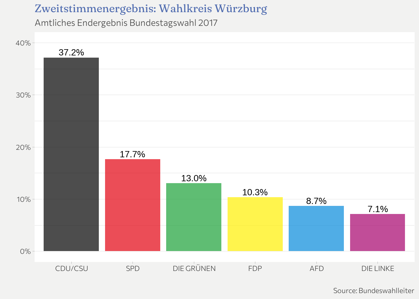
A quick look at website confirms: the numbers match!
Next we join the election results for each Wahlkreis with the corresponding geometry information of that Wahlkreis. Once this is done, we can plot a map all 299 German Wahlkreise and color each according to a given party’s share of valid votes. Since we have done all the work already, joining is easy now.
election_matched <- wahlkreise_shp_2017 %>%
  left_join(election_cleaned, by = c("WKR_NR" = "Wahlkreis_nr"))
To check if there are any mismatches, I always simply do an anti-join which returns everything that didnt get matched.
# Check if everything got matched
wahlkreise_shp_2017 %>%
  anti_join(election_cleaned, by = c("WKR_NR" = "Wahlkreis_nr"))
## Simple feature collection with 0 features and 4 fields
## Bounding box:  xmin: NA ymin: NA xmax: NA ymax: NA
## Geodetic CRS:  WGS 84
## [1] WKR_NR    WKR_NAME  LAND_NR   LAND_NAME geometry
## <0 rows> (or 0-length row.names)
Perfect! No mismatches. To be able to plot the map + election results for each party without repeating code a little function is handy:
plot_election_results <- function(party, color_high) {
  election_matched %>%
      filter(Party == party) %>%
      ggplot(aes(fill = Results)) +
      geom_sf() +
      scale_fill_gradient(high = color_high, low = "white",
                          labels = scales::label_percent(scale = 1)) +
      labs(
         title = "Bundestagswahl 2017",
         # the term inside the {} is evaluated an inserted when exectued. See ?glue
         subtitle = glue::glue("Zweitstimmen der {party} in %"),
         fill = ""
         # caption = "Source election results: Bundeswahlleiter\nSource map: Bundesamt für Kartographie und Geodäsie"
      ) +
      theme(
         panel.background = element_rect(fill = "white", colour = "white"),
         plot.background = element_rect(fill = "white", colour = "white"),
         legend.background = element_rect(fill = "white", colour = "white"),
         axis.title = element_blank(),
         axis.text = element_blank(),
         axis.ticks = element_blank(),
         panel.grid.major = element_blank(),
         legend.position = "bottom"
      )
}
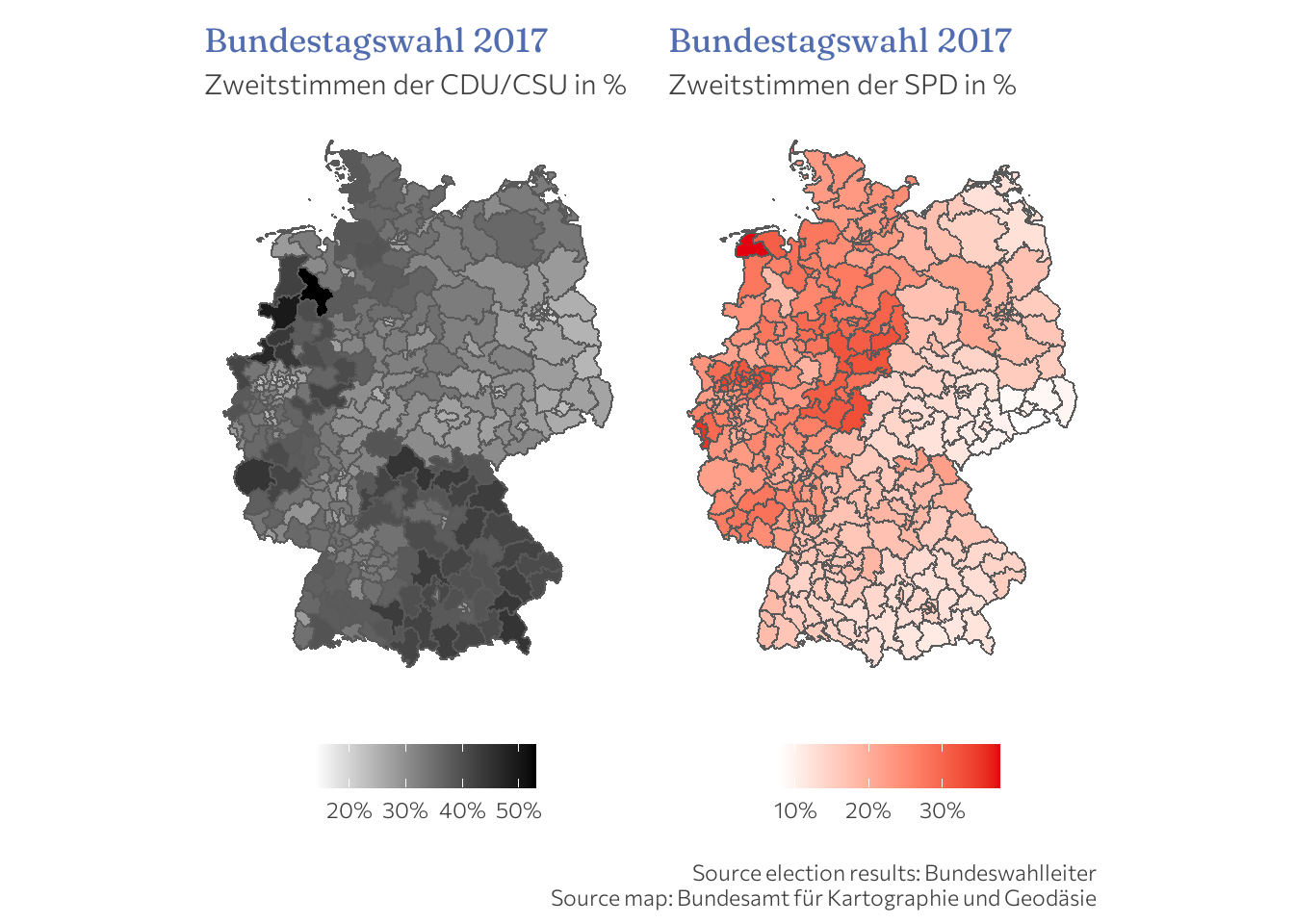
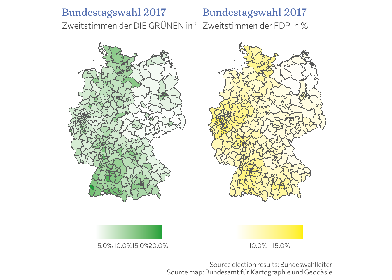
Now, we are finally ready to reproduce the figure on the left side of the KATAPULT graphic as well as those for the other parties.
a <- plot_election_results("CDU/CSU", color_high = party_colors["CDU/CSU"])
b <- plot_election_results("SPD", color_high = party_colors["SPD"])
a + b  +
   plot_annotation(
      caption = "Source election results: Bundeswahlleiter\nSource map: Bundesamt für Kartographie und Geodäsie"
      ) &
   theme(plot.background = element_rect(fill = "white", colour = "white"))
a <- plot_election_results("DIE GRÜNEN", color_high = party_colors["DIE GRÜNEN"])
b <- plot_election_results("FDP", color_high = party_colors["FDP"])
a + b +
   plot_annotation(
      caption = "Source election results: Bundeswahlleiter\nSource map: Bundesamt für Kartographie und Geodäsie"
      ) &
   theme(plot.background = element_rect(fill = "white", colour = "white"))
a <- plot_election_results("AFD", color_high = party_colors["AFD"])
b <- plot_election_results("DIE LINKE", color_high = party_colors["DIE LINKE"])
a + b +
   plot_annotation(
      caption = "Source election results: Bundeswahlleiter\nSource map: Bundesamt für Kartographie und Geodäsie"
      ) &
   theme(plot.background = element_rect(fill = "white", colour = "white"))
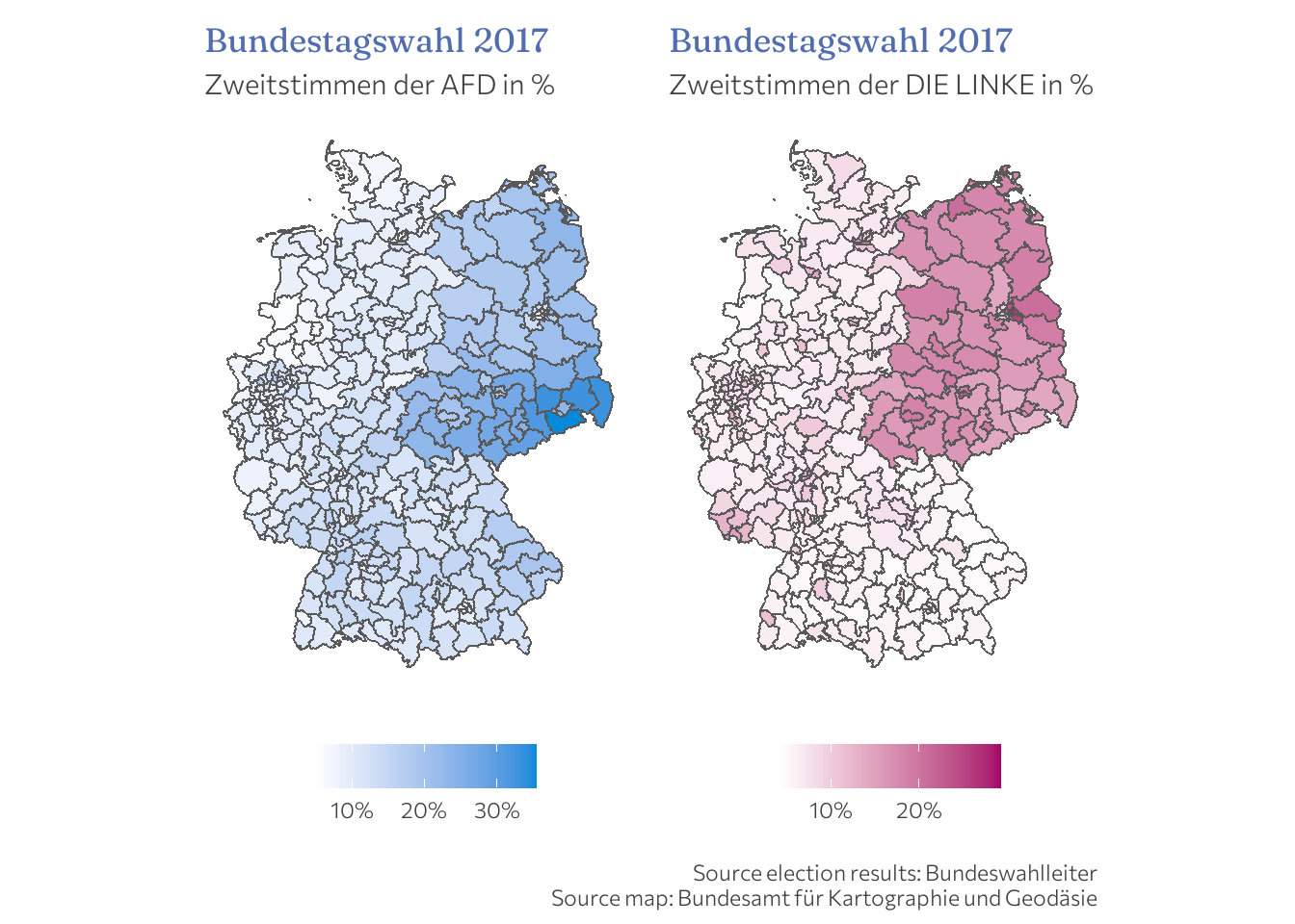
While there are many things to notice, its particularly striking to see how well AfD and DIE LINKE are doing in the new Bundesländer – and how bad the other parties perform there – compared to the rest of Germany. If you ever need a visualization to stress that the Wiedervereinigung has still not been finished… here you go!
Adding interactivity
Static maps are fine, but who does not like interactivity? There are many ways to achieve
interactivity. If you are comfortable around ggplot and are fine with some basic
interactivity tools like a tooltip, the
ggiraph package is
probably most easiest to pick up. You simply switch the regular geom_* or scale_*
objects from ggplot with their interactive counterpart from ggiraph and subsequently
wrap the whole plot in the girafe() function. That’s basically it.
For illustration, lets make the AfD map interactive. To make it even more like
the original figure, I also added binned results.
afd_plot <- election_matched %>%
   filter(Party == "AFD") %>%
   # simplify the geometry: the interactive map embeds every vertex in the page,
   # at full resolution the page would be ~11 MB
   rmapshaper::ms_simplify(keep = 0.02, keep_shapes = TRUE) %>%
   # Add binned election results according to the bins of the original figure
   mutate(
      Results_binned = cut(Results,
                           breaks = c(4.9, 10, 15, 20, 25, 35.5),
                           labels = c("4,9 bis 10", "bis 15", "bis 20", "bis 25", "bis 35,5"))
   ) %>%
   ggplot() +
   # use the interactive version and add a tooltip; glue comes in very handy here!
   geom_sf_interactive(aes(fill = Results_binned,
                           tooltip = glue("Wahlkreis: {Wahlkreis}\nResult: {scales::percent((Results/100), accuracy = 0.01)}"))) +
   scale_fill_brewer(palette = "Blues") +
   labs(
      title = "Bundestagswahl 2017",
      # the term inside the {} is evaluated an inserted when executed. See ?glue
      subtitle ="Zweitstimmen in Prozent (AfD)",
      fill = "",
      caption = "Sources: Bundeswahlleiter; Bundesamt für Kartographie und Geodäsie"
      ) +
   theme(
      panel.background = element_rect(fill = "white", colour = "white"),
      plot.background = element_rect(fill = "white", colour = "white"),
      legend.background = element_rect(fill = "white", colour = "white"),
      axis.title = element_blank(),
      axis.text = element_blank(),
      axis.ticks = element_blank(),
      panel.grid.major = element_blank(),
      legend.position = "bottom"
      )

girafe(ggobj = afd_plot)
Incidence by Landkreis
In the next step we focus on infection data, most notably the 7-day incidence by Landkreis.
First, based on the raw RKI data, we produce a clean data set with
only three columns: AGS (the Landkreis Id), Date and Cases. The latter column
is the absolute number of cases. In a next step, we
need to join the cleaned data with the vg250_ew_2020 data set which provides the
population info per Landkreis required to compute the incidence.
The RKI infection data is provided in a relatively clean form, however, the structure takes a bit to get used to – at least I think so. Lets take a look:
infections_raw %>% head(8) %>% gt()
| IdLandkreis | Altersgruppe | Geschlecht | Meldedatum | Refdatum | IstErkrankungsbeginn | NeuerFall | NeuerTodesfall | NeuGenesen | AnzahlFall | AnzahlTodesfall | AnzahlGenesen |
|---|---|---|---|---|---|---|---|---|---|---|---|
| 1001 | A15-A34 | M | 2020-10-28 | 2020-01-19 | 1 | 0 | -9 | 0 | 1 | 0 | 1 |
| 1001 | A15-A34 | M | 2020-03-19 | 2020-03-13 | 1 | 0 | -9 | 0 | 1 | 0 | 1 |
| 1001 | A15-A34 | M | 2020-03-21 | 2020-03-13 | 1 | 0 | -9 | 0 | 1 | 0 | 1 |
| 1001 | A35-A59 | M | 2020-03-14 | 2020-03-16 | 1 | 0 | -9 | 0 | 1 | 0 | 1 |
| 1001 | A15-A34 | M | 2020-03-19 | 2020-03-16 | 1 | 0 | -9 | 0 | 1 | 0 | 1 |
| 1001 | A15-A34 | M | 2020-03-14 | 2020-03-16 | 1 | 0 | -9 | 0 | 1 | 0 | 1 |
| 1001 | A35-A59 | M | 2020-03-20 | 2020-03-17 | 1 | 0 | -9 | 0 | 1 | 0 | 1 |
| 1001 | A60-A79 | M | 2020-03-26 | 2020-03-19 | 1 | 0 | -9 | 0 | 1 | 0 | 1 |
Each row is a group of cases (“Fallgruppe”) possibly containing several cases!
A group is uniquely identified by the variables AnzahlFall, Altersgruppe, Geschlecht,
IdLandkreis, Meldedatum, Refdatum, and IstErkrankungsbeginn.
We are interested in the AnzahlFall column.
What makes this data a bit confusing at first are the three columns NeuerFall, NeuerTodesfall, and NeuGenesen
which constitute the report status (“Meldestatus”). These are used to indicate
whether a new group (row) is a correction to some other group compared to the that
groups status on the previous day or simply a new case group (NeuerFall = 0).
Corrections can be negative or positive (indicated by a -1 or + 1 in the NeuerFallcolumn).
These correction – to my surprise – can even refer to cases many month back in time. For example, using todays data (as of writing this “today” means: 2021-08-31) Landkreis with Id = 5382 reported a correction to a case with a Meldedatum as old as 2020-05-28.
infections_raw %>%
   filter(NeuerFall == 1) %>%
   arrange(Meldedatum) %>%
   head(6)
## # A tibble: 6 x 12
##   IdLandkreis Altersgruppe Geschlecht Meldedatum Refdatum   IstErkrankungsbeginn
##         <dbl> <chr>        <chr>      <date>     <date>                    <dbl>
## 1        5382 A35-A59      W          2020-05-28 2020-05-26                    1
## 2        9178 A35-A59      W          2020-09-14 2020-09-09                    1
## 3        9178 A35-A59      M          2020-09-15 2020-09-15                    0
## 4       16077 A15-A34      M          2020-10-08 2020-10-08                    0
## 5       16077 A60-A79      W          2020-10-25 2020-10-25                    0
## 6       16077 A35-A59      W          2020-10-26 2020-10-26                    0
## # ... with 6 more variables: NeuerFall <dbl>, NeuerTodesfall <dbl>,
## #   NeuGenesen <dbl>, AnzahlFall <dbl>, AnzahlTodesfall <dbl>,
## #   AnzahlGenesen <dbl>
Therefore, the RKI data is considered a prime data set when looking at past numbers: you can be sufficiently sure that every correction to the numbers ever reported to the RKI are reflected in this data set.
On the downside, it may not be the best data if you need up-to-data near-real-time data.
Luckily, for our purpose things like “Meldeverzug” and past vs. real-time data are
not a particular big issue since if NeuerFall is not 0 (indicating a normal report),
the variable AnzahlFall has the respective sign of the NeuerFall column.
Simply summing the absolute numbers by Landkreis and Meldedatum takes thus care
of any corrections giving the exact number of infections reported to the RKI including
all past corrections ever made.
infections <- infections_raw %>%
  select(IdLandkreis, Altersgruppe, Geschlecht, Meldedatum, AnzahlFall) %>%
  group_by(IdLandkreis, Meldedatum) %>%
  summarise(AnzahlFall = sum(AnzahlFall)) %>%
  ungroup()

infections %>% head(6) %>%  gt()
| IdLandkreis | Meldedatum | AnzahlFall |
|---|---|---|
| 1001 | 2020-03-14 | 4 |
| 1001 | 2020-03-18 | 2 |
| 1001 | 2020-03-19 | 4 |
| 1001 | 2020-03-20 | 2 |
| 1001 | 2020-03-21 | 1 |
| 1001 | 2020-03-24 | 1 |
A couple of things remain to be addressed.
-
As stated in the README on the RKI GitHub page > Für eine genauere Darstellung des Landkreises Berlin, werden die 12 Stadtbezirke als eigene “Landkreise” aufgegliedert (For a more accurate representation of the Berlin district, the 12 districts are broken down as separate “Landkreise.”)
To easily join the cases and the population/geometry data sets we need to take care of that. Since I’m not interested in the details of each district of Berlin, we simply aggregate the 12 districts and give them the Berlin AGS label.
-
For some reason the Landkreis Id does not match the AGS exactly. All IdLandkreis < 10000 should actually have a leading zero. This needs to be fixed for proper matching.
infections <- infections %>%
   # filter the 12 Berlin districts and summarize numbers by Meldedatum
   filter(IdLandkreis %in% 11001:11012) %>%
   group_by(Meldedatum) %>%
   summarise(AnzahlFall = sum(AnzahlFall)) %>%
   # create new column IdLandkreis with only the value 11000 (AGS for Berlin)
   mutate(IdLandkreis = 11000) %>%
   # Bind the Berlin rows back into the "main" data (with the individual Berlin districts removed)
   bind_rows({infections %>% filter(!(IdLandkreis %in% 11001:11012))}) %>%
   # arrange by Landkreis and Meldedatum
   arrange(IdLandkreis, Meldedatum) %>%
   # Fix the missing leading zero in IdLandkreis and rename to AGS
   group_by(IdLandkreis, Meldedatum) %>%
   mutate(AGS = if_else(IdLandkreis < 10000, paste0(0, IdLandkreis), as.character(IdLandkreis))) %>%
   # cleanup
   ungroup() %>%
   select(-IdLandkreis) %>%
   relocate(AGS)
7-day incidence
The 7-day incidence per 100’000 people in each Landkreis on a given date is the rolling 7-day sum over the absolute number of positive cases (only PCR test!) of that Landkreis and date divided by the total population per 100’000 of the Landkreis.
To compute the rolling sum, the zoo::rollsum() can be used. Let’s compute the
rolling sum, join the population/geometry data and lastly compute the incidence per 100’000
people. I also compute the 7-day rolling mean to be able to plot a smooth
curve of total infections below.
Note that technically the 7-day rolling sum (and mean) at the beginning of the
reporting are not correctly computed by roll* as e.g., rollsum() simply moves from observation to observation,
takes the last 7 observations (assuming they are ordered) and computes the sum.
At the beginning reportings did not come in on a daily basis leading to a rolling
sum longer than a 7-day period. This issue, however, is minor since these reporting
gaps only happened at the beginning of the pandemic.
As far as the population/geometry data set is concerned a small modification is
necessary – which I missed at first. Currently, there are 401 Landkreise and kreisefreie Städte
in Germany. However, the data set vg250_ew_2020 contains 431 rows.
The reason is the variable DEBKG_ID. Column DEBKG_ID allows for easy joining to
another data set called “Digitalen Landschaftsmodell” (DLM250) provided by the
Bundesamt für Kartografie und Geodäsie which contains objects such as roads, rails etc.
Apparently, one (Land)Kreis can have multiple DEBKG_IDs. If a Kreis has
multiple DEBKG_ID it appears in multiple lines of the vg250_ew_2020 data set.
Hence the additional 30 rows.
However, population is set to 0 for any appearances but the first in the data.
Since we only require the geometry and the population, we have to delete all appearances
of a Kreis that have EWZ (the population) equal to zero. Failing to delete those rows
leads to double matching once we join the two data sets. As a consequence, case numbers
would be counted twice inflating the number of actual cases.
infections_with_geometry <- vg250_ew_2020 %>%
   # remove doubled rows
   filter(EWZ > 0) %>%
   # select only relevant columns
   select(AGS, Landkreis_name = GEN, EWZ, geometry) %>%
   # join in the infections data
   left_join({
      infections %>%
         group_by(AGS) %>%
         # see ?rollsum for what fill = NA does
         mutate(
            seven_day_rollmean = zoo::rollmeanr(AnzahlFall, k = 7, fill = NA),
            seven_day_rollsum  = zoo::rollsumr(AnzahlFall, k = 7, fill = NA)
         )
   }, by = "AGS") %>%
   # compute 7-day incidence
   mutate(Infections_per_100k = seven_day_rollsum / (EWZ/1e5)) %>%
   ungroup()
Thats it! As usual its a good idea to check if everything went as expected. Plotting the absolute number of new COVID-19 cases by reporting date for Germany as a whole is a good first indication. Again we add interactivity in order to allow for a easy comparison to the numbers of the official RKI dashboard. In this case, we use the dygraph library which is an R interface to the dygraphs JavaScript charting library. The reason is simple: its super easy to use and yet supports the essentials of interactivity like zooming in on a date range and hovering. There is even a little box on the left bottom that allows for computation of a rolling mean. Enter e.g. 7 and you get the 7-day rolling mean.
infections_plot <- infections_with_geometry %>%
   tibble() %>%
   select(AGS, Meldedatum, AnzahlFall) %>%
   group_by(Meldedatum) %>%
   summarise(Cases = sum(AnzahlFall))


# dygraph requires an xts object
xts_series <- xts(x = infections_plot$Cases, order.by = infections_plot$Meldedatum)

# Create an R wrapper for the barplott plotter
dyBarChart <- function(dygraph) {
  dyPlotter(dygraph = dygraph,
            name = "BarChart",
            path = system.file("plotters/barchart.js",
                               package = "dygraphs"))
}

dygraph(xts_series, main = "New COVID-19 cases in Germany by reporting date") %>%
   dyBarChart() %>%
   dyRangeSelector()  %>%
   dyCrosshair(direction = "vertical") %>%
   dyAxis("x", drawGrid = FALSE) %>%
   dyAxis("y", label = "# Cases") %>%
   dyRoller(rollPeriod = 1)
Alright, manual inspection shows that the numbers do match almost everywhere.2 There are slight differences towards the newest dates. I think the reason is that the data that get uploaded to RKI’s GitHub page is not exactly identical to the data underlying the dashboard.
Now, we are ready to reproduce the figure from the start of this post. Remember, the snapshot date was 2020-12-18.
NOTE: For some reason, I cant get more than two interactive plots to work when deploying this post to the web server. Locally, it works but when clicking on the post just as you did a couple of minutes ago, the blog post incorrectly ends here. All plots are therefore static now, but you can simply uncomment the interactive sections in the code below to have it run interactively on your local machine.
infections_plot <- infections_with_geometry %>%
   filter(Meldedatum == "2020-12-18") %>%
   # Add bins
   mutate(
      Infections_per_100k_binned = cut(Infections_per_100k,
                           breaks = c(25, 50, 100, 250, 500, 1000),
                           labels = c("über 25\nbis 50", "über 50\nbis 100", "über 100\nbis 250", "über 250\nbis 500", "über 500\nbis 1.000"))
   ) %>%
   ggplot() +
   # use the interactive version and add a tooltip; glue comes in very handy here!
   # geom_sf_interactive(aes(fill = Infections_per_100k_binned,
   geom_sf(aes(fill = Infections_per_100k_binned)) +
   scale_fill_brewer(palette = "OrRd") +
   labs(
      title = "Fälle letzte 7 Tage pro 100.000 Einwohner",
      fill = "",
      caption = "Sources: RKI GitHub; Bundesamt für Kartographie und Geodäsie\nStand: 18.12.2020."
   ) +
   theme(
      panel.background = element_rect(fill = "white", colour = "white"),
      plot.background = element_rect(fill = "white", colour = "white"),
      legend.background = element_rect(fill = "white", colour = "white"),
      axis.title = element_blank(),
      axis.text = element_blank(),
      axis.ticks = element_blank(),
      panel.grid.major = element_blank(),
      legend.position = "bottom"
   )
# interactive version
# girafe(ggobj = infections_plot)
infections_plot
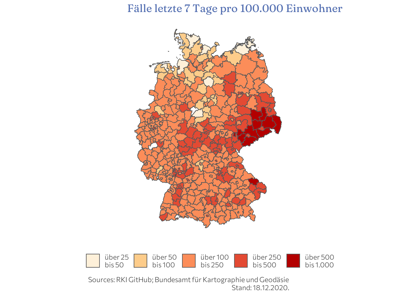
If you look closely, you see that some Landkreise are dark red, i.e. category “über 500 bis 1.000” (e.g. Erzgebirgekreis, SN) in our figure while in the original KATAPULT figure they are one category below. I guess the difference is simply due to reporting corrections. As already mentioned, the RKI has its strength in the past. A cross-check with e.g. this dashboard confirms that the more recent numbers in our figure are correct.
Do 2017 AfD election results predict the 7-day incidence
This is already a long post, however, now comes the interesting part. Lets see if there is some more compelling evidence for the implied hypothesis that AfD election results are predictive for the 7-day incidence. The most critical issue with the election result-to-incidence graphic is of course the date: 2020-12-18. During the pandemic cases went up and down, Landkreise whose numbers skyrocket found themselves with neglectable numbers a couple of month later while other Landkreise started to suffer.
Much more telling than a simple one-day snapshot is evolution over time by party stronghold. The biggest issue is that it is actually pretty tedious to match Wahlkreise and Landkreise. As I mentioned at the beginning: Walhkreise (of which there are 299) do follow the Landkreis boundaries if possible but differ on many significant occasions. The reason is simple: Wahlkreise ought to be “similar” in terms of number of voters etc.
Seeing that the AFD performed strongest in Sachsen and parts of Thüringen a rough quick-and-dirty approximation is to simply take these two Bundesländer as a proxy for “AFD stronghold.”
Let’s plot the 7-day incidence for these who Bundesländer (i.e. the AFD stronghold) over time and compare to the incidence of the rest of the country.
infections_with_geometry %>%
   tibble() %>%
   select(AGS, Meldedatum, AnzahlFall, EWZ) %>%
   mutate("Area" = if_else(startsWith(AGS, "14") | startsWith(AGS, "16") , "AFD stronghold (SN & TH)", "Rest of the Germany")) %>%
   group_by(Area, Meldedatum) %>%
   summarise(Cases = sum(AnzahlFall), Population = sum(EWZ)) %>%
   mutate(
      seven_day_rollsum  = zoo::rollsumr(Cases, k = 7, fill = NA),
      Infections_per_100k = (seven_day_rollsum / Population)*1e5
      ) %>%
   ggplot(aes(x = Meldedatum, y = Infections_per_100k, color = Area)) +
   geom_line() +
   scale_color_manual(values = c("AFD stronghold (SN & TH)" = unname(party_colors["AFD"]), "Rest of the Germany" = "green")) +
   labs(
      title = "7-day incidence per 100.000 people over time",
      x = "",
      y = ""
   )
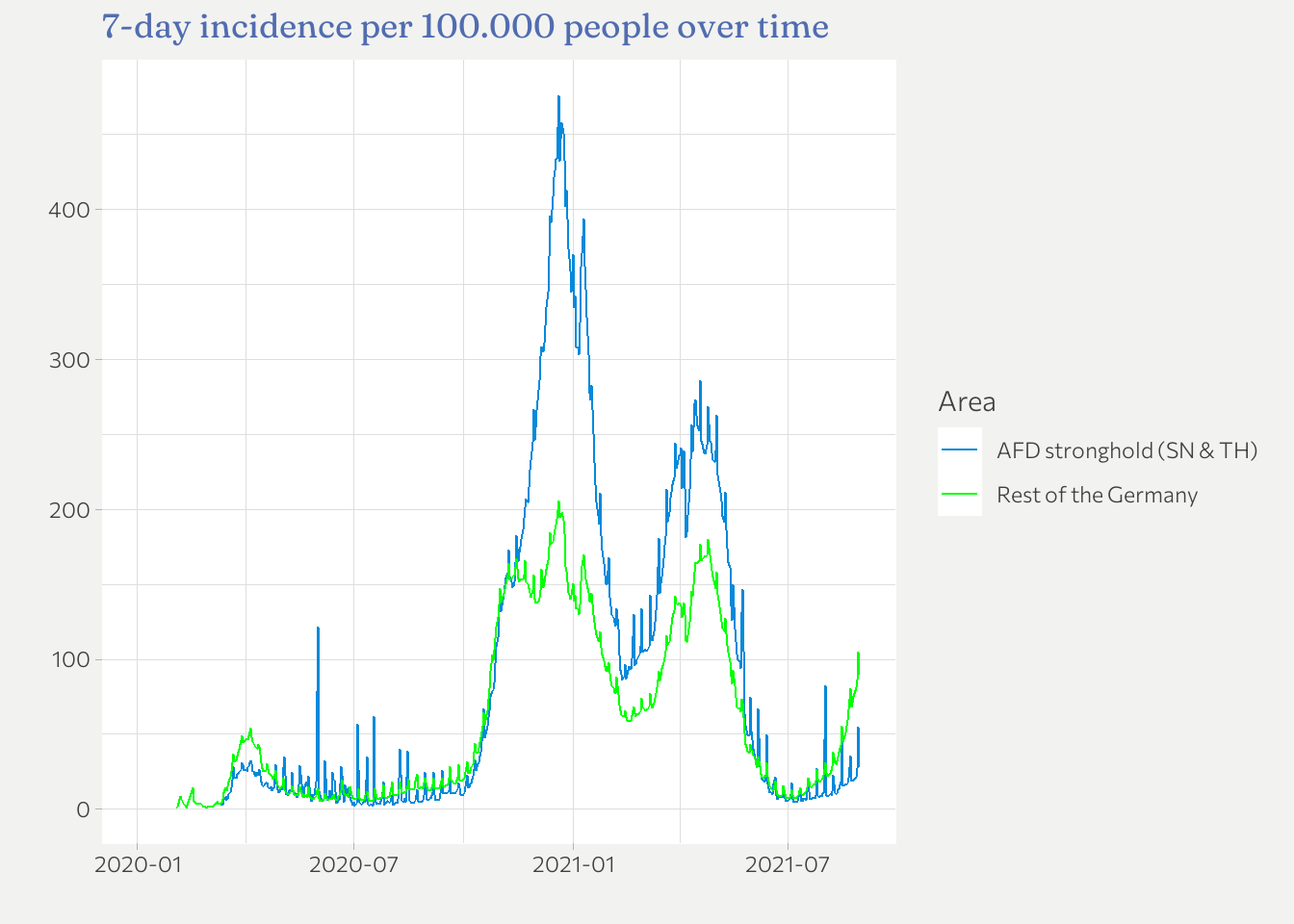
The figure suggests a correlation indeed, in particular, during the worst times of the pandemic. On the other hand, the most recent numbers indicate a strong upward movement in the numbers in the rest of Germany. Remains to be seen if the AFD strongholds catch up.
I do not want to get into a causal analysis here because that requires a much, much more detailed look at the numbers and, hence, a separate blog post. However, the correlation is definitely reason for thought.
Vaccination by Landkreis
Lastly, I want to briefly discuss vaccination data. As I wrote at the beginning, it would be highly interesting to see if there is a similar correlation to election results when using the vaccination rate per Landkreis. Well, that’s simply not possible right now.
The reason is that vaccination centers, hospitals, doctors etc. only report
the location they gave a vaccination shot (usually simply the zip code
of their address) but not where the vaccinated person actually lives!
An obvious problem: people are not required to get vaccinated in the same area
as their own zip code, so Landkreise with vaccination centers are likely to have
much higher vaccination rates compared to those that don’t. Consequently, “Vaccination by Landkreis”
is actually rather misleading. To illustrate the severity of the problem, lets
naively compute the vaccination rate by Landkreis by simply dividing the
sum of vaccinations administered in a given Landkreis by the population of
that Landkreis.
## Compute total by day, Landkreis and vaccination dose (1 or 2)
vaccinated <- vaccinated_raw %>%
   rename(AGS = LandkreisId_Impfort) %>%
   # sum over all age groups
   group_by(Impfdatum, AGS, Impfschutz) %>%
   summarise(Anzahl = sum(Anzahl)) %>%
   # sum over all day
   group_by(AGS, Impfschutz) %>%
   summarise(Geimpft = sum(Anzahl)) %>%
   ungroup()

vaccinated %>% head(6) %>%  gt()
| AGS | Impfschutz | Geimpft |
|---|---|---|
| 01001 | 1 | 79658 |
| 01001 | 2 | 73921 |
| 01002 | 1 | 184382 |
| 01002 | 2 | 168164 |
| 01003 | 1 | 148412 |
| 01003 | 2 | 141709 |
The “u” in the AGS columns stands for “unknown Landkreis.” I delete all observations that don’t belong to a Landkreis.
vaccinated <- vaccinated %>%
  filter(AGS != "u")

# Let's check if there are 401 Kreise
length(unique(vaccinated$AGS))
## [1] 402
Turns out there are 402 Landkreise. A quick look in the documentation on the RKI GitHub website reveals. There is an additional “Landkreis” with number 17000 which comprises all Bundesressorts. I am not exactly sure what a “Bundesressort” is, but since we are not interested in the overall vaccination rate, we can drop those.
vaccinated <- vaccinated %>%
  filter(AGS != 17000)
Next, we need to join population data and geometry information
vaccinated_matched <- vg250_ew_2020 %>%
   # remove doubled rows
   filter(EWZ > 0) %>%
   # select only relevant columns
   select(AGS, Landkreis_name = GEN, EWZ, geometry) %>%
   left_join(vaccinated, by = "AGS") %>%
   mutate(
      vaccination_rate = Geimpft / EWZ
   )
And here is the plot. Again, enable interactivity by uncommenting the interactive code parts.
vaccination_plot <- vaccinated_matched %>%
   # Remove "Auffrischungsimpfungen"
   filter(Impfschutz %in% 1:2) %>%
   mutate(Impfschutz = if_else(Impfschutz == 1, "Einmal geimpft (ex Janssen)", "Voll geimpft (incl. Janssen)")) %>%
   ggplot() +
   # use the interactive version and add a tooltip; glue comes in very handy here!
   # geom_sf_interactive(aes(fill = vaccination_rate,
   #                         tooltip = glue("Landkreis: {Landkreis_name}\nVaccintion rate: {scales::percent(vaccination_rate, accuracy = 0.1)}"))) +
   geom_sf(aes(fill = vaccination_rate)) +
   scale_fill_gradient(low = "white", high = party_colors["DIE GRÜNEN"],
                       label = scales::label_percent()) +
   facet_grid(cols = vars(Impfschutz)) +
   labs(
      title = "'Vaccination rate' by Landkreis",
      subtitle = "WARNING: vaccination rate based on where the vaccine was given, \nnot (!) the zip-code of the vaccinated person.",
      fill = "",
      caption = "Sources: RKI GitHub; Bundesamt für Kartographie und Geodäsie\nStand: 2021-08-31"
   ) +
   theme(
      panel.background = element_rect(fill = "white", colour = "white"),
      plot.background = element_rect(fill = "white", colour = "white"),
      legend.background = element_rect(fill = "white", colour = "white"),
      axis.title = element_blank(),
      axis.text = element_blank(),
      axis.ticks = element_blank(),
      panel.grid.major = element_blank(),
      legend.position = "bottom"
   )

# Interactive version.
# girafe(ggobj = vaccination_plot)
vaccination_plot
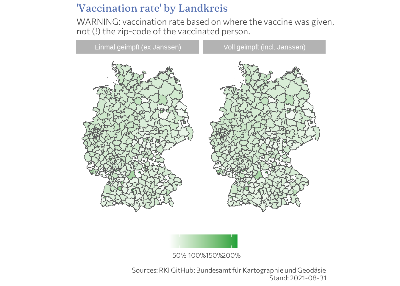
As you can see, there are some Landkreise (in particular kreisefreie Städte, which are very likely to have a vaccination center) with vaccination rates above 100% – a clear indicator that numbers should not be interpreted as the vaccination rate of those that life in that Landkreis.
-
Technically, its the first 16 rows of the original data with the first 5 rows skipped. ↩︎
-
When you read this post, the numbers on the dashboard will be for the current date. Numbers of the newer dates are therefore likely to differ compared to the ones of this post, since, as already mentioned, correction to previous reportings affect previously reported numbers. ↩︎
- Posted on:
- August 31, 2021
- Length:
- 69 minute read, 14534 words
- Categories:
- Data Science Covid 19 SARS-COV2 2017 Election R Maps Interactivity
- See Also: